2023 Edition

Agriculture & Natural Resources
Download (PDF)

Share this Newsletter

Additional Newsletters

Preview This Newsletter

Russell County Agriculture and Natural Resources Sept. - Oct. Newsletter

Jonathan Oakes, CEA for Agriculture and Natural Resources

Upcoming Events: 
September 14: BQCA Training@ Russell Co. Ext. Office @ 5:30pm 
September 15-16: KY Wood Expo @ Masterson Station Park- Lexington, KY- Call for more information 

September 21: UK Beef Bash- Versailles, KY- Call our office for more information 
September 23: Hunter Education Course @ Russell County Sportsman's Club­. Must register online 
September 25: Rinse and Return and Agriculture Chemical Take-back Day@ Russell County Ext. Office from 9-llam 
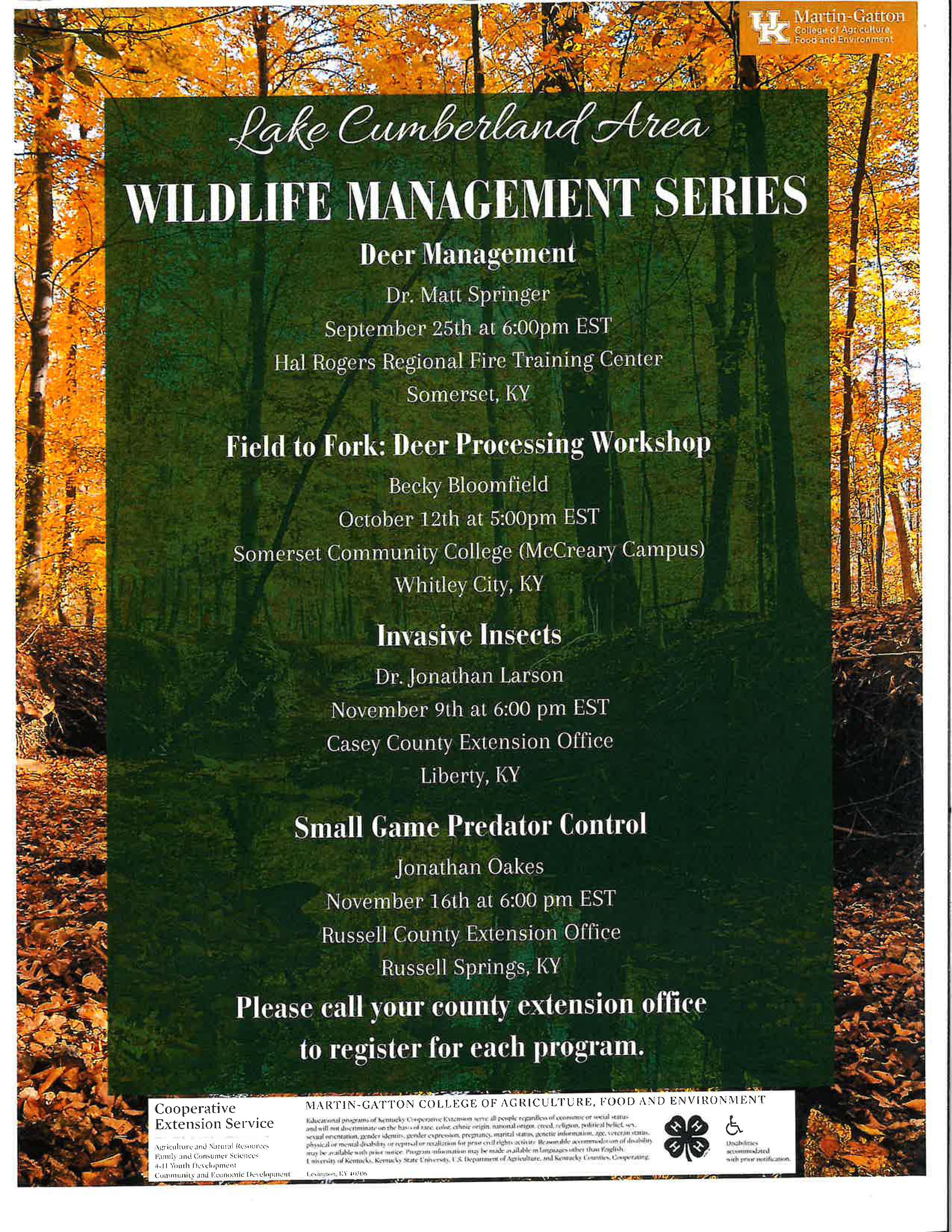
September 25: Lake Cumberland Area Wildlife Series Session 1 @ Pulaski County @Spm CST- see attached flyer 
September 28: BQCA Training@ Russell County Ext. Office @ 5:30pm 
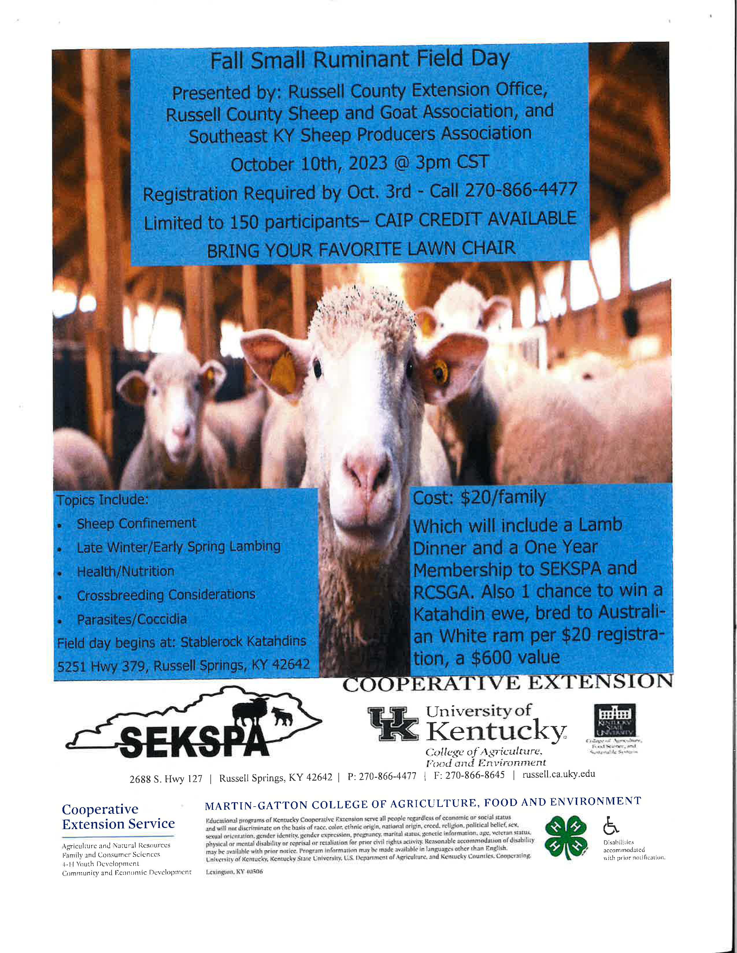
October 10: Small Ruminant Fall Field Day@ Stablerock Katahdins @ 3pm CST­ see attached flyer 
October 12: Lake Cumberland Area Wildlife Series Session 2 @ McCreary County @ 4pm CST- see attached flyer 
October 19: KSU Third Thursday- Small Ruminant Workshop @ KSU Research Farm 

Future of Beef Production May be Up in the Air

Jeff Lehmkuhler, Extension Professor, University of Kentucky 

A couple of weeks ago, the national meeting of the American Society of Animal Science was held. This is a professional organization that many of us in the animal sciences field are members of for professional development. Several of us from the University of Kentucky attended to present research, learn about on-going research, teaching and extension activities from other states and receive awards. In my opinion, the impact of animal agriculture on climate change is a key focus of current research at many institutions. In a search of the agenda, 25 presentations and 23 posters were presented when I conducted a search using the term methane. Let me put that in context, when I searched using just the term antibiotic, only 9 presentations and 7 posters were found. Though a variety of information was shared covering numerous topics, the number of papers focused on the impact of animal agriculture on climate change couldn't be ignored. 
In an invited presentation, Dr. Al Rotz, USDA researcher, shared information related to greenhouse gas emissions (GHG) from beef cattle operations. This team published a life cycle assessment for GHG for beef cattle in 2019 and a comprehensive assessment in 2023 that was partially funded by Beef Checkoff dollars. The authors reported the model estimated the current amount of feed required to produce 1 kg (2.2 lbs.) of carcass weight of beef was approximately 22 kg (44 lb). This is a feed conversion efficiency of 22:1 while you often hear of feed efficiency rates of 5 to 6: 1 for live weight gain in the feedlot sector. Using 62% dressing percentage, a 6: 1 feed-to-gain ratio would be roughly 10: 1 if we expressed it on a carcass weight basis. Automatically, you should be getting red flag warnings and calling this work BS. However, this was a full life cycle assessment, womb to tomb if you will. The authors point out that the cow­calf sector accounts for nearly 73% of the feed inputs in the beef production system while the stocker/background and finishing phases accounted for 10% and 17%, respectfully. 
Dr. Rotz in his presentation stated that beef production accounts for approximately 3.5% of the national GHG emissions. Their work further reported on emissions, energy and water use as well. The cow-calf sector was shown to contribute roughly 77% of the methane emissions. Beef animals are essentially walking fermenters, consuming forage and feed in which ruminal organisms get the first opportunity to ferment producing carbon dioxide, methane, ammonia and other compounds. This is what makes cattle unique in that they can utilize feeds that are non­edible by humans and convert these into high quality protein. The authors further broke down the beef systems by region. The southeast was reported to have the greatest weighted average GHG emissions. 
As part of the Paris agreement, the United States committed to reducing GHG by 50-52% by 2030. With respect to agriculture, the 2021 US Long Term Strategy document discusses the protection and increase of forested areas. Data reported by EPA indicate that beef cattle emitted 22% of the total agricultural GHG emissions. The increase in practices that are referred to as 
"climate-smart" which includes the use of cover crops and rotational grazing as examples will receive greater emphasis in the future. 

In Rotz's presentation in Albuquerque, he shared that food waste accounted for 20-30% of the GHG emissions in the U.S. which exceeded the proportion from beef production system of 3.5%. The global food waste contribution to GHG emissions reported by FAQ using 2011 estimates was 3.3 gigatonnes of carbon dioxide equivalents (GtCO2e). In their recent 2023 publication, Rotz and co-authors state "The magnitude of this impact makes waste (food) one of the greatest impacts on environmental sustainability." Consider all the inputs to produce food are accounted for in the production chain and when food is wasted carbon emissions still occur. How much food is thrown out in your household, large community gatherings or when we dine out? How many vegetables and packages of meat are tossed from the grocery stores due to exceeding expiration dates? Food waste is also a distribution challenge on a global scale. 
For nearly a decade, we have been hosting the Kentucky Beef Efficiency Conference. The information shared directly relates to our ability to reduce GHG and global warming potential 
( G WP) by the beef industry. Remember the cow-calf sector is the greatest contributor to G WP in the beef system. Combining knowledge with management change to reduce waste is a first step. 
Waste in my mind is equal to production losses. Redirecting our focus to increasing beef produced per unit of land will be needed. Additionally, the cow-calf sector will need to focus on increasing pounds of beef weaned per cow exposed. I am not advocating for maximizing, but rather optimizing. Increasing reproductive rates and weaning percentage should be an initial focus. Many factors contribute to these areas. Conducting breeding soundness exams, pregnancy checking to reduce feed inputs to non-productive cows, and improving our forage base to maintain body condition on cows to ensure breeding and increasing stocker performance will aid in reducing beefs carbon footprint. Reducing death losses through improved immunization is a very simple step. Where possible pasture renovation to novel endophyte tall fescue or interseeding clover will improve forage utilization and reduce GHG per pound of beef produced. There are several management tools in our toolbox that play a role in reducing the climate impact of beef production. These steps will also improve financial sustainability in the long run. 
Making strides forward now as an industry will reduce the chance of policy intervention. The tabloids are full of European headlines discussing meeting climate change goals through the reduction of animal populations. Becoming informed and knowledgeable on sources of GHG emissions will also aid you in discussing with consumers what you are doing to reduce your carbon footprint and what they can do as well. How we will progress as an industry to lessen our GWP remains up in the air for now, but you can be assured this will not be going away anytime soon. 

Information for Beef Bash 

Tyler Purvis, Beef Extension Associate, University of Kentucky 

It's that time of year again! Beef Bash will be held Thursday, September 2ist from 2 p.m. to 8 p.m. at the C. Oran Little Research Center. Dinner will be provided by the Woodford County Cattleman's Association at 5 p.m. Pre­registration for attendees will be $15 and includes a meal ticket. Come out to see all the latest UK research, interact with extension specialists, and browse a variety of vendors. 

Yield Monitor Maps for P and K Fertilizer Rate Prescription Maps??

Developing a field's variable rate fertilizer prescription map can be costly, including the time in taking plant tissue and/or soil samples, sample analysis costs, and later map development time. Soil sample analysis is particularly important to phosphorus (P), potassium (K) and soil acidity (pH) management. Soil sampling time may be in short supply when crop harvest is to be followed by es­tablishment of a succeeding crop. Soil test results are not always timely, further delaying prescrip­tion map development. Due to the expense, grid or zone sampling is often done only every 2 to 4 years, which raises the question of how much fertilizer is to be applied in other years. 

Other precision technologies, especially yield maps, are being used to reduce the time crunch. Ferti­lizer prescription maps based on nutrient removal can be developed directly from a yield map by multiplying the yield by grain P or K concentration values taken from published tables. Intuitively, nutrients would be applied to replace nutrients removed by the previous crop. A random sample of the grain could be analyzed if values from published tables were thought inappropriate. 
There are potential problems with this approach. Limiting factors other than nutrient deficiency, especially water stress (both too little and too much), can drive field yield patterns. Should this year's insect/disease pressure or weed competition patterns drive fertilizer P and K application? If a low soil test P limits crop yield in one area, should that area then be fertilized according to the low P removal found with the low yielding, P deficient, crop? The yield monitor map might improve fer­tilizer prescriptions, but how does it compare with other options? 
We compared four approaches to generating field-scale fertilizer rate prescriptions: a) the "grid", based on (expensive) grid soil sampling a field on a 180 x 200 ft. grid (about 1 sample per 0.83 acre) and spatial analysis of the soil test results; b) the "composite", based on a single average soil test value from all grid soil samples taken in the field; c) "yield map nutrient removal-tabular", based on the field's yield map, a single published grain P concentration value, and spatial analysis of the cal­culated nutrient removal values; and d) "yield map nutrient removal-local composite", based on the field's yield map, a single grain P concentration value determined on a composite grain sample tak­en from that field, and spatial analysis of calculated nutrient removal. 
Two producer fields, designated 112 (51.4 ac) and 950 (43.4 ac), were chosen. The dominant soil in both fields was a well-drained Crider silt loam, but there were sizeable areas of only moderately well drained soil (Lowell, Nicholson or Tilsit silt loams). Field 112 had a history of chemical fertiliz­er applications and 950 had a history of swine manure and fertilizer N applications. Corn yield was determined with a calibrated yield monitor. Grain and soil samples were taken at the same grid point, shown in Figure 1A for field 950. A digital elevation map was determined for each field (also shown in Figure 1A for field 950). Soil test P was determined by the Mehlich III extraction proce­dure at the University of Kentucky's Division of Regulatory Services soil test laboratory. This lab also determined soil pH and organic matter on each soil sample. Grain tissue was analyzed for P by the University of Kentucky Plant and Soil Sciences Department's Analytical Services Laboratory. 
Maps were generated for crop yield/nutrient removal and soil test P. The tabular value used to cal­culate nutrient removal maps was 0.326 % P = 0.353 lb P2Os/bu. Table 1 shows the fertilizer rate prescription as related to P removal or soil test P values. 

Fertilizer Prescription (lbs. P2O5/ac)	Removal (lbs./ac) (lbs. P2O5/ac)	Soil Test P (lbs./ac)
0	0-15	>60
30	15-45	42-60
60	45-75	28-42
90	75-105	14-28
120	105-135	0-14

Table 1. Fertilizer prescriptions as related to removal or soil test values

 

"Composite" soil test, grain yield and grain tissue P information for the two fields are given in Table 2. On average, field 950 was higher in soil test P and organic matter, but soil pH values were similar. Grain yield was lower, and more variable, in 112 than 950. For 950, grain P was close to the tabular value, and grain from 112 was lower than the tabular value.

Property	Field 950	Field 112
Soil Test P (lb/ac)	147 ± 64	54 ± 31
OM(%)	3.3 ± 0.6	2.6 ± 0.4
pH	6.4 ± 0.3	6.3 ± 0.6
Yield (bu./ac)	138 ± 22	130 ± 47
Grain P (%)	0.35 ± 0.03	0.29 ± 0.04

Table 2. Soil test, yield, and grain composition information for each field (mean± one standard deviation). 

The soil test P map for field 112 (not shown) also showed considerable spatial variation. Comparing prescription approaches for this field, fertilizer P is over-prescribed, relative to that recommended by "grid" sampling, by both nutrient removal approaches (Table 4 ). In 112, the greater difference be­tween the grain P concentration value for grain taken from the field and the value taken from the ta­ble caused the removal-based fertilizer P prescriptions to differ. The "composite" soil analysis recom­mended a uniform rate of 30 lbs. P2O5 per acre for field 112. 

Relative to grid soil sampling, the "composite" P rate prescription was appropriate for a third of the field, over-fertilized a third of the field, and under-fertilized a third of the field (Table 4). 

Fertilizer Prescription  (lbs. P2O5/ac)	Grid Soil Test P (%)	Composite Soil Test P (%)	Removal Tabular Grain P (%)	Removal-Local Composite Grain P (%)
0	100	100	0	0
30	0	0	38.4	23.3
60	0	0	61.7	76.7
90	0	0	0	0
120	0	0	0	0

Table 3. Portion (in %) of field 950 receiving each fertilizer P rate, according to the prescription method. 

Fertilizer Prescription  (lbs. P2O5/ac)	Grid Soil Test P (%)	Composite Soil Test P (%)	Removal Tabular Grain P (%)	Removal-Local Composite Grain P (%)
0	30.5	0	0	0
30	36.0	100	43.1	74.1
60	31.7	0	56.5	25.9
90	1.7	0	0.5	0
120	0	0	0	0

Table 4. Portion (in %) of field 112 receiving each fertilizer P rate, according to the prescription method.

We concluded that composite soil sampling was not always inferior to grid soil sampling in terms of the resulting fertilizer P or K prescriptions, especially when both approaches confirmed that no ferti­lizer was needed. In general, using yield-nutrient removal maps to derive fertilizer prescription maps resulted in greater prescribed P and K fertilizer rates than either soil test approach. We also observed that as the tabular grain P concentration value deviated from the field grain P concentration there was more of a difference in the nutrient removal-based fertilizer P prescription. Our results indicate that using yield monitor maps and grain P or K concentration information to develop variable rate fertiliz­er P and K rate prescription maps rests upon an assumption that was often not valid. We found P and K removal by the most recently harvested crop is not better related to the need for fertilizer P and K for the next crop than current soil test P and K values. 

That said, our experience indicates that yield maps can be used, along with soil, topographic and other spatial information (satellite imagery) to divide a field into "management zones" that better capture crop production differences than simple square/rectangular grids. These zones, likely few­er, would then be soil sampled for nutrient management information. •

Co-authors: 
Dr. John Grove, Professor of Agronomy /Soils Research and Extension, University of Kentucky 
Dr. Eugenia Pena-Yewtukhiw, Assoc. Professor, Soil Physics and Management, Director, WVU Soil Test­ing Laboratory, West Virginia University, Morgantown, WV  

 

What Do Higher Profit Farms in Kentucky Have in Common? 
Author(s): Lauren Omer Turley 
Published: August 29th, 2023 

In today's farming culture, the farm is run just as a business. It is important for producers to make progress and always look for ways to improve the operation. The goal of most producers is to be at the top of the profitability curve in order to stay competitive. In Kentucky, we have had a record three­-year period from 2020 to 2022. There were excellent yields combined with decent prices and low input costs. Everything combined resulted in very positive net farm incomes over the period. Looking at the current year, the 2023 crop, input costs have risen drastically and commodity prices are 
lower. Yields are still unknown, but this will most likely be a year of tight margins although producers' efficiencies are being maximized. Crop yields do play a major factor in management returns; however, the diversity of the operation also has an impact. It is interesting to examine the characteristics of the higher profit farms over the past five years. 
Data from the Kentucky Farm Business Management program for 2018 through 2022 were used to analyze differences between the highest profit grain farms (high one-third) and the lower profit grain farms (low one-third). The analysis was done for 2022 and for the 2018 through 2022 five-year average on a per acre basis. Farms in the higher profit group were larger, had higher corn and soybean yields, cash rented a larger percentage of their acres, had a larger percentage of their acres in corn, and had higher gross returns and lower costs. Management returns, a profit measurement, were significantly greater for the higher profit farms. Management returns are calculated using gross returns, cash costs, economic (rather than tax) depreciation, and imputed costs for interest and owner labor. 

Table 1: Differences Between High and Low Thirds - 2022

Com Yield (bu.)	17
Soybean Yield (bu.)	9
Operator Tillable Acres	1,117
% Owned	- 6 %
% Crop Share	4 %
% Cash Rent	2 %
Gross Farm Returns	$267
Crop Costs	($20)
Power & Equipment Costs	($16)
Total Economic Costs	($65)
Management Returns	$324
% Acres Corn	6 %
% Acres Soybeans	- 1 %

Table 2: Differences Between High and Low Thirds - 5-Year Average

Com Yield (bu.)	15
Soybean Yield (bu.)	5
Operator Tillable Acres	1,215
% Owned	0 %
% Crop Share	- 7 %
% Cash Rent	7 %
Gross Farm Returns	$229
Crop Costs	($16)
Power & Equipment Costs	($26)
Total Economic Costs	($78)
Management Returns	$314
% Acres Corn	5 %
% Acres Soybeans	-10 %

Farm size was a consistent factor in the profitability, as the higher profit farms were 574 acres to 1640 acres larger than the lower profit farms over the five-year period. In 2022, livestock returns (primarily poultry) were a factor in the higher profit farms. Beef cattle also had positive returns in 2022, which was a change from the past five years. The larger farms are able to spread the fixed costs over more acres. Over the five-year period, the average difference in farm size was 1215 acres. This is a large difference as the average size of the farms only ranged in size from 1261• acres to 2920 tillable acres. 
Another consistent factor of the higher profit farms was yield. Both corn and soybean yields were higher over the five years. As the table shows, for the five-year average, corn yield was 15 bushels higher and soybean yield was 5 bushels higher. This would obviously result in higher gross returns per acre. In 2022, their yield advantage was a considerable 17 bushels for corn and 9 bushels for soybeans. Weather is one major contributor to the higher yields, but management practices also impacted the yields across the state. The higher profit farms also had a larger percentage of their tillable acres planted in corn and less in full season soybeans. More corn acres will also add to the higher gross farm returns as an acre of corn will produce more returns than an acre of soybeans. 
Management practices also impact the costs. The crop costs include seed, chemicals, and 
fertilizer. An acre of corn is more expensive than an acre of beans, thus one would assume the costs should be higher for the farms that have a larger percentage of their land in corn. However, crop costs for the higher profit farms (with a larger percentage of their land in corn) were $16 lower than the lower profit farms on average over the five-year period. Less inputs to generate higher returns resulted in these farms being at the top. In 2022, the crop costs were $20 lower per acre for the higher profit farms. The largest crop input factor over the past five years, and most likely for the 2023 crop as well, was fertilizer. In 2022, on an average grain farm, crop input costs have been 35-40% of total costs. It is difficult to reduce overall costs when such a large percentage of costs are tied up in inputs that really can't be reduced without impacting gross returns. Input prices have been very volatile over the last year, thus monitoring input costs has been a top priority for producers. 
As expected, the higher profit, larger farms had lower power and equipment costs. This category includes utilities, equipment repairs, fuel, machine hire and lease, and equipment economic depreciation. The largest costs are repairs, machine hire, and economic depreciation. Spreading these costs over more acres allows for more efficiency. Total economic costs include crop costs, power and equipment costs, building costs, labor costs, miscellaneous costs, and land costs. In 2022, total costs were $65 per acre lower for the higher profit farms, which you can see over half of that difference is a result of crop and equipment costs. In 2022, labor was $36 more for the lower profit farms. One reason for this is more tobacco on the lower profit farms. Tobacco is labor intensive and since the lower profit farms were smaller, there were fewer acres to spread the labor costs across. Economic costs were $78 less for the five-year average, and 54% of that difference is a result of crop and equipment costs. 

Another interesting factor to discuss is the ownership and rental agreements of the higher profit farms. Different areas of the state have primarily different rental agreements. Some landlords prefer cash rent and a guaranteed set price, while other landlords are willing to take a risk for higher returns and possibly share in some crop expenses. In 2022, the higher profit farms owned 6% less of their land, crop shared 4% more of their land, and cash rented 2% more of their land. The average cash rent for these farms was only $203, a very economical cash rent. Over the five-year period, the average difference for the higher profit farms was crop sharing 7% less, and cash renting 7% 
more. With the economical cash rent average, the crop share farms have been a larger cost to the producers over the period. 
The larger gross farm returns and the lower costs have resulted in significantly larger management returns for the higher profit farms. In 2022, the higher profit farms averaged $324 more per acre in management returns. Over the five-year period the average difference was $314 per acre. 

There are many factors that contribute to the profitability of the farms. Some factors, such as weather, cannot be controlled, but the management practices of each operation impact many other factors. Forward planning and knowing breakeven costs are more important now than in the 
past. With the volatilities of the commodity markets and the fertilizer markets, producers should be aware of their costs in order to "pull the trigger" when the time comes. Not one single factor will be the consistent main contributor to the difference in profitability. The goal.of all producers should be to analyze personal trends and work toward improving their individual operation. 
If you would like more information about the Kentucky Farm Business Management program, please contact one of the specialists in your area. 

Turley, L. O. "What Do Higher Profit Farms in Kentucky Have in Common?" Economic and Policy Update (22):7, Department of Agricultural Economics, University of Kentucky, August 29th, 2023. 

Author(s) Contact Information: 
Lauren Omer Turley I KFBM Area Extension Specialist I lauren.o.turley@uky.edu 

 

2023 Farm Bill Completion Remains in Limbo as Congress Returns from its August Recess 
Author(s): Will Snell 
Published: August 29th, 2023 

This past month Congress has been on its annual August recess and will be returning after the Labor Day holiday to begin the charge to pass a new farm bill. The current 2018 farm bill expires on September 30, 2023. In the midst of anticipated lower future prices for most ag commodities, higher borrowing costs, and reduced ad hoc government outlays for farmers, the ag community is urging Congress to pass this ongoing piece of legislation that has been in place since the New Deal programs of the 1930s. However, upon its arrival back to our nation's capital, Congress faces a host of appropriation bills that must be passed to keep the government running after September 30th which will likely take on a lot of valuable floor debate and ultimately slow down the progress of a new farm bill. In total, there are only 11 scheduled legislative days when both chambers will be in session during the entire month of September. Although both the Senate and House ag committees have conducted numerous hearings on developing a new farm bill, neither body has "marked up" a bill and passed a bill in committee to deliver to the floor for consideration. So, the bottom line is don't anticipate passage of the 2023 farm bill prior to the September 30th deadline. Even without a new farm bill by September 30th, many farm bill programs such as farm commodity and dairy support, crop insurance, and nutrition programs will continue with a more pressing deadline of passing a new farm bill before December 31, 2023. (Click here for more details.) While leadership within the ag committees remains optimistic that Congress can send a new farm bill to the President for his signature prior to the end of the year, many challenges loom moving forward. 
In reality, not many new issues have evolved since I provided my last update in this newsletter back in late April. (Click here to see the article). Most of the debate has continued to center around crop insurance, reference (safety-net) prices, conservation programs, trade promotion, and of course food assistance programs (i.e., food stamps/SNAP). Traditionally passage of a farm bill has benefited from bipartisan support which will once again be critical to getting this one across the finish line. However, there are plenty of differences on issues across and even within political parties on general farm support and nutrition program structure, eligibility, and funding. Plus, there is the usual debate on equity of program support across commodities and geographical regions. 
Funding remains a key challenge moving forward as various agricultural groups are requesting increases in reference prices to offset higher input costs along with additional risk management coverage for specialty crops and livestock enterprises. Environmentalists are seeking additional dollars for expanded conservation programs and technical support. Nutrition supporters are demanding to maintain/increase food assistance for low-income households challenged by this economy. Increases in funding various farm bill programs will likely have to be offset with decreases in funding for other programs as established by the farm bill baseline. If the ag committees can come to an agreement on the components and the funding levels to pass a bill out of committee, then one can likely expect a host of amendments to evolve once the bill hits the Senate and House floors where a block of members on both sides of the aisle have some concerning differences on the 
"appropriate" level of taxpayer dollars to fund an estimated $1.5 trillion farm bill amidst on-going federal debt/deficit challenges. 
Over the past two months, there has also been a lot of attention within the farm bill debate to 
the concept of "base" acres which are used in the calculations of payments for the two primary safety net programs (Price Loss Coverage (PLC) and Agricultural Risk Coverage (ARC)) for eligible crops (primarily corn, wheat, and soybeans for Kentucky). Base acres within the current farm bill were established over two decades ago and were tied to historical plantings and not to current planted acres. This policy action is designed to allow U.S. producers to make their cropping decisions based on current market conditions and not in response to anticipated government payments. This so-called "decoupling" of the cropping decisions also passes the scrutiny of the World Trade Organization (WTO), the international body that plays referee on policies impacting trade. As a result of policy structure, farmers with eligible base acres can actually receive payments on crops for which they no longer plant. 
Given the changes in cropping patterns over the years there are a significant number of planted acres that are not eligible for farm bill safety net payments. This is especially true for soybeans in our state where Kentucky has a tad over 900,000 base acres of soybeans, but in recent years planted around 1.9 million acres of soybeans. Some of these acres might have shifted from one program crop such as wheat to soybeans (and thus retain price/income protection), but there are likely a significant number of farms in Kentucky that have shifted out of livestock or some other non-farm bill enterprise such as tobacco into grain production after the establishment of historical base acres eligible for farm bill payments. The 2014 farm bill did allow farmers a one-time adjustment to reallocate base acres within program crops, but not to increase their total level of base acres. 
A recent Senate Ag Committee analysis indicates that Kentucky would be one of 16 states that would benefit from a mandatory update in base acres. However, according to the analysis, the majority of U.S. states would likely observe farm bill payment losses as eligible base acres shift to crops with a lower degree of support within the farm bill. In total, the study indicates a net loss approaching $2 billion with a new mandatory realignment of base acres. While this action could free up some dollars for other farm bill programs/safety net measures, as with any significant policy change there will be winners and losers which may threaten overall support for dramatic changes in the current farm bill structure given anticipated tight vote margins expected to pass a new farm bill. 
So hang on for some heated debate and creative budget/policy maneuvers to construct a potential passable farm bill within the next few months ... or simply an extension of the 2018 farm bill. 

Snell, W. "2023 Farm Bill Completion Remains in Limbo as Congress Returns from its August Recess." Economic and Policy Update (23):8, Department of Agricultural Economics, University of Kentucky, August 29th 2023. 

Author(s) Contact Information: 
Will Snell I Extension Professor wsnell@uky.edu 

Wildfire Preparedness 
By Simone Lewis - National Weather Service Charleston, WV

When the word wildfire comes to mind, images of burning forests in the western United States usually enter the thoughts of most. But did you know that Kentucky is also prone to wildfires? In fact, the state averages 1,447 wildfires a year! The following article will discuss what weather conditions are favorable for wildfire development, the weather alerts that are issued during periods of favorable fire weather, and what you can do to prepare for and prevent wildfires. 

The first question on your mind is probably "What is Fire Weather"? Essentially, fire weather is any sort of weather that can ignite or lead to rapid spread of fires. This includes thunderstorms (which contain strong gusty winds and lightning that can lead to rapid spread or ignition of a fire), days when the relative humidity is low (often in the early spring and fall seasons), and windy days (which acts to not only spread wildfires but also leads to the drying of vegetation, making it more susceptible to burning). 

Wildfire Prevention

Most wildfires in the state of Kentucky are caused from arson or from uncontrolled debris burning. In fact, 90% of all wildfires in Kentucky are caused by humans. Unlike many fires in the western United States, most of the fires in Kentucky are fought by firefighters on the ground (Source: Kentucky Energy and Environment Cabinet). They are putting their lives in danger to control the spread of these fires. It is therefore important to always be fire aware, and heed any Fire Weather Watches or Red Flag Warnings issued by the NWS.

Here are some general guidelines to follow when the following products are issued: 

Fire Weather Watch = BE PREPARED! Dangerous fire weather conditions are possible in the next few days but are not occurring yet. 

Red Flag Warning = Take Action! Dangerous fire weather conditions are ongoing or expected to occur shortly. During a Red Flag Warning, you should avoid or use extreme caution when dealing with anything that could pose a fire hazard. 

• Do not start a campfire or ignite a burn pile.
• Do not burn trash.
•  Avoid using a lawnmower, chainsaw, or any other equipment that may emit sparks.
• Do not dispose of cigarette butts on the ground or outside of your car.
•  If using an outdoor grill, make sure to have a water source nearby and do not dispose of the ashes until the Red Flag Warning has expired or been canceled AND the ashes are fully extinguished!
• Watch for smoke nearby. If you spot an unattended fire, call 911 and report it immediately!

What do I do to prepare?

Take personal responsibility by preparing long before the threat of a fire, so your home and family are ready. 

•    If there are concerns of fire potential, create a defensible space by clearing brush that is easier to ignite away from your home.
•    Put together a basic emergency supply kit. Check emergency equipment, such as flashlights and generators.
•    Plan escape routes and make sure all those residing within the home know the plan of action.
•    Sit down with your family and close friends, and decide how you will get in contact with each other, where you will go, and what you will do in an emergency. Keep a copy of this plan in your emergency kit, or another safe place where it can be accessed in the event of an emergency.
•    Review your insurance policies to ensure that you have adequate coverage for your home and personal property in the event of fire.
•    Follow the latest NWS forecasts and listen to a NOAA Weather Radio for the latest updates.

What are Kentucky's Fire Laws?

Lastly, it's important to know and heed the fire laws and seasons for the state of Kentucky. During the following periods, it is illegal to burn anything within 150 feet of any woodland or brushland between the hours of 6 a.m. and 6 p.m. 

•    Spring Forest Fire Hazard Season: February 15 - April 30
•    Fall Forest Fire Hazard Season: October 1 - December 15

Also, burn bans can be issued at any time of the year if conditions warrant, particularly during periods of drought, and should always be followed. 

Tracking the First Fall Freeze 
by Derrick Snyder - National Weather Service Paducah, KY

As the calendar moves into October, nights continue to become longer, leaves begin to turn color, and first frosts and freezes begin to occur. The first freeze of the fall typically marks the end of the growing season. As shown on the map below, most locations across the Commonwealth typically see their first freeze of the season during the latter half of October into the early days of November. 

Frost can often develop on plants even when thermometers show the temperature to be a few degrees above freezing. This is because most thermometers are mounted several feet above the ground, and the temperature a few inches from the ground can be colder than what a thermometer reads. These most often occurs on clear nights with calm winds. 
To protect your plants from frosts and freezes, consider taking preventive measures like covering them with tarps or blankets in the evening before temperatures drop. This can help trap the ground heat and provide insulation. Additionally, placing mulch around the base of plants can help retain soil warmth. If possible, relocate potted plants indoors or to a sheltered area. Watering the plants before the onset of frost can also provide a slight protective effect, as water releases heat as it freezes, helping to moderate the immediate environment around the plants. 

 

 

 

 

 

 

 

 

 

 

 

 

 

 

 

 

 

 

 

 

 

 

 

 

 

 

 

 

 

 

 

 

 

 

 

 

 

 

 

 

 

 

MARTIN-GATTON COLLEGE OF AGRICULTURE, FOOD AND ENVIRONMENT

Educational programs of Kentucky Cooperative Extension serve all people regardless of economic or social status 
and will not discriminate on the basis or race, color, ethnic origin, national origin, creed. religion, political belief sex, sexual orientation, gender identity, gender expression, pregnancy, marital status, genetic information, age, veteran status, physical or mental disability, or reprisal or retaliation for prior civil rights activity. Reasonable accommodation of disability may be available with prior notice. Program information may be made available in languages other than English. University or Kentucky, Kentucky State University, U.S. Department or Agriculture, and Kentucky Counties, Cooperating. 
Lexington, KY 40506.